Financing the LBO: Part I

Today we begin the first part of a two-part series on Leveraged Buyouts ("LBOs"). This opening piece sets the stage with an overview of the practice and its mechanics. In part two, we will dive into the calculations behind the main instruments used to finance an LBO and put them all together in a debt schedule.

The structure of this chapter will be as follows: (1) a historical overview of the origins and development of LBOs, (2) the mechanics of how they are executed by their usual employers i.e., private equity funds ("Sponsors"), (3) a short discussion of how these investors seek to generate returns, (4) an outline of the typical companies that are suitable LBO candidates, and finally (5) a more theoretical but essential discussion of how LBOs fit within capital structure.ture.

For readers approaching this for the first time, certain concepts may appear unclear. We are not building every piece of theory from scratch. Instead, the focus is on what is directly relevant for understanding LBOs. For example, when comparing outcomes, I will use IRR without unpacking the full mechanics, with the simple note that, generally, a higher IRR is better. Likewise, in discussing capital structure, I will not go into every detail of the calculations, but rather highlight the elements that matter most for costs.

Let's dive in.

SOME HISTORY

Early Roots (1950s - 1960s)

The idea of financing acquisitions with borrowed money has roots well before the term “LBO” was coined. In the mid-1950s, McLean Industries, Inc. issued $7 million in preferred shares on top of $42 million of its own equity to acquire Pan-Atlantic Steamship Company. Other deals followed a similar model of layering external capital on top of equity, including Warren Buffett’s use of outside investors in his acquisition of Berkshire Hathaway. Still, in hindsight, many of these early transactions do not meet the definition of a modern LBO.

Consolidation of the Concept (1970s)

It was not until the late 1970s that the leveraged buyout began to take shape in its modern form. Henry Kravis and his cousin Jerome Kohlberg, then at Bear Stearns, described these early efforts as “bootstrap” investments—a phrase later chronicled in Merchants of Debt by B. Anders, which traces the origins of KKR. Over time, the industry settled on a working definition: an LBO involves a sponsor firm, a temporary investment horizon with a planned exit, and more than half of the purchase price financed with debt. By this standard, many of the earlier deals from the 1960s fall outside the category, despite their superficial resemblance.

The First Boom (1980s)

The practice gained rapid momentum in the 1980s with the emergence of the high-yield bond market, pioneered by Michael Milken at Drexel Burnham Lambert. Junk bonds allowed deals to be financed on a scale that had previously been impossible, culminating in the iconic RJR Nabisco buyout, later immortalized in Barbarians at the Gate. At the same time, regulatory changes encouraged corporations to spin off divisions, while the cultural backlash against “management extravagance” reinforced the view that many firms were underperforming due to weak incentives. The result was a wave of corporate takeovers, often hostile, that defined the decade. But by the early 1990s the cycle collapsed. Excessive leverage left many firms with fragile balance sheets, leading to widespread defaults. The reckoning was compounded by Milken’s indictment for financial crimes, which ended Drexel’s dominance and marked the first true crisis in the LBO market.

The Era of "Mega-LBOs" (2000s)

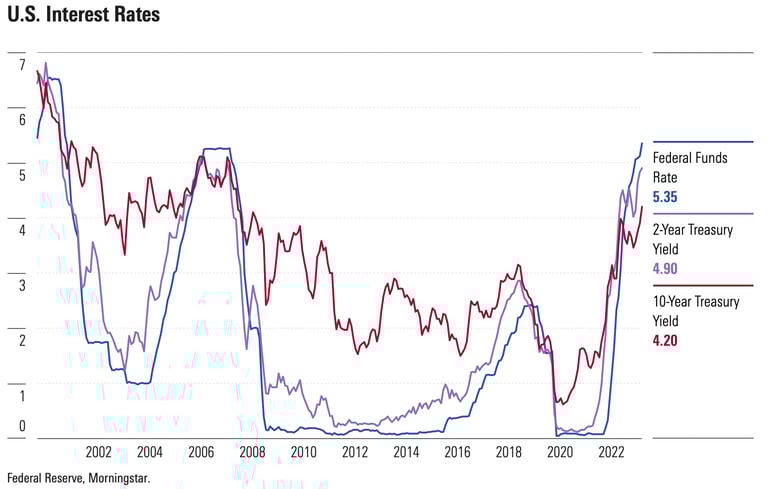
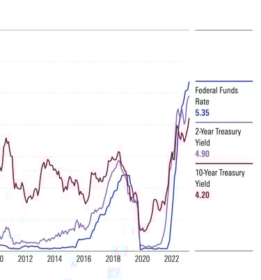
After a quieter late 1990s, the next wave emerged in the 2000s amid a backdrop of steadily declining interest rates. This became the era of the “mega-LBO,” with transactions financed at unprecedented scale. The most notorious example was the buyout of TXU by KKR and TPG, which ultimately collapsed into one of private equity’s largest failures. During this period, new financing techniques such as payment-in-kind (PIK) instruments also spread, allowing sponsors to defer cash interest and further stretch capital structures.

Crisis and Recovery (2008-2010s)

The boom ended abruptly with the 2008 financial crisis, when credit markets froze and deal-making came to a standstill. In the aftermath, LBO activity resumed, but at more moderate sizes. Sponsors became more cautious, reflecting lessons about the dangers of overextension. Yet the following decade nonetheless turned into another golden age, fueled by persistently low interest rates. For those who deployed capital in the immediate post-crisis years, the period delivered some of the strongest private equity returns in recent memory.

Pattners from History

Now, the reason why I provided this historical background wasn't to entertain the reader with general culture or nostalgia, but to emphasize that LBOs do follow as well cycles broadly related to macro and market conditions from where certain patterns can be observed which might allow one to get a sense on where the LBO market may be directed in the next years. As such, a few patterns from the past decades of LBOs stand out:

1. Credit Availability and Interest Rates: LBOs usually are abundant in abundant credit periods and low borrowing costs. The rise of junk bonds in the 1980s, the falling rate environment of the 2000s, and the post-GFC decade of ultra low-interest rates each enabled a surge in buyout activity. Conversely, when credit markets tighten - whether in early 1990s or during the 2008 financial crisis - LBO volume collapses. 

2. Financial Innovation: New instruments tend to unlock new waves of activity. In the 1980s, high-yield bonds made large-scale deals feasible. In the 2000s, payment-in-kind (PIK) notes and covenant-lite loans gave sponsors more flexibility, though also encouraged risk-taking. Innovation expands the market, but also plants the seeds for excess

3. Regulatory and Structural Shifts: Each cycle has been supported by regulatory backdrops that made deal-making easier. In the 1980s, looser rules around divestitures allowed corporations to spin off divisions. In the 2000s, a more permissive credit environment let banks and institutional investors distribute risk broadly.

4. Corporate Culture: Perceptions about underperformance and inefficiency create fertile ground for buyouts. The critique of “management extravagance” in the 1980s or the narrative of “unlocking value” in conglomerates both fueled waves of LBOs. Cultural narratives often align with financial conditions to justify higher activity.

5. Cycle of Overreach and Correction: Every expansion has been followed by a contraction. Excessive leverage in the late 1980s triggered defaults in the early 1990s. The mega-deals of the 2000s collapsed into the GFC. Even the post-GFC boom, while highly profitable, reflects the same pattern: abundant credit fuels growth until conditions change.

THE MECHANICS OF AN LBO

Now that we are somewhat familiar with the origins of the LBO, its core concept (borrowing to fund an acquisition), and its primary practitioners (private equity sponsors), it is worth turning to the practical side. In practice, sponsors usually begin with a high-level “LBO valuation.” At this stage, they take the company’s financial statements as given, apply assumptions on leverage and returns, and test whether the business might fit their strategy or meet their target IRR. The deeper, more granular analysis—where assumptions are refined, bankers get involved, and deal structuring takes place—comes later in the private equity deal process, once the target is under serious consideration. In other words, LBO discussions sit somewhere in the middle of the deal timeline, as shown below. Below is a usual PE analysis and deal process and the LBO might sit somwhere in the middle of the process.

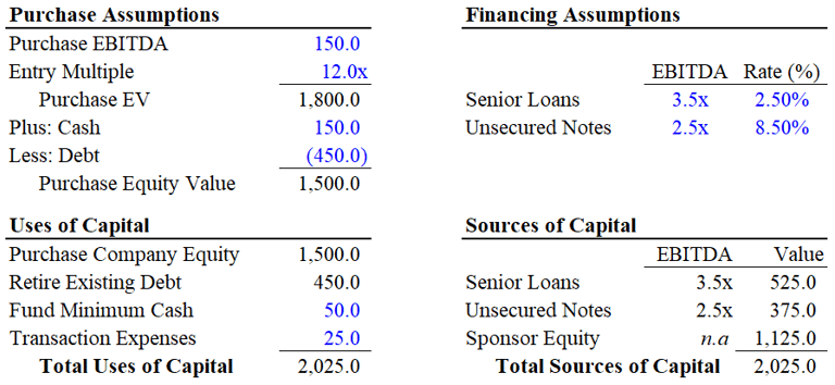
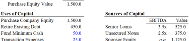
When the company engages lenders in this financing step (the fourth box in the sequence), the sponsor finally gets a clearer view of two critical things: (i) the actual cost of debt, and (ii) how receptive the credit markets are - meaning the supply and demand for different instruments and the yields attached to them which allows a more precise calculation on the cost of debt to fund the acquistion. At this point, a “Uses and Sources” table is either put together, so the sponsor can see exactly how much equity he must contribute. Such a table usually resembles the one from below: 

In this example, the Sponsor has to put 55.5% of the purchase price, which albeit perfectly possible if the business is risky or has revenue or cash flow fluctuations and the sponsor has conviction it, albeit usually would be only 40-20% of equity i.e. "Sponsor Equity".

To clarify, the Uses and Sources table is simply a way to match what the deal costs (Uses) with where the money comes from (Sources). It can be sketched early on, but at this later stage it becomes much more complete. For example, lenders may indicate that, beyond the loan initially considered, the market is open to absorbing unsecured bonds. Professional fees (lawyers, advisors, bankers) are more precisely estimated. And most importantly, due diligence provides a clearer sense of the company’s fair price, which may adjust the sponsor’s assumptions. All of these inputs feed into the Uses and Sources table, making it a fairly precise picture of how the deal will actually be funded.

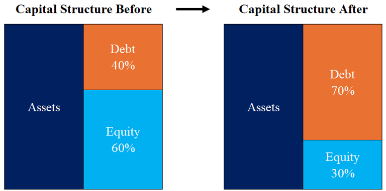
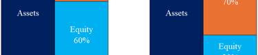
Now, assuming the transaction goes through and the sponsors succeed in acquiring the company, the capital structure will be reshaped to reflect the new layer of debt placed on top of the existing liabilities. In other words, the balance sheet is re-levered, with debt now accounting for a much larger share of the financing mix, as shown below:

WHAT DRIVES LBO RETURNS

When we looked at the origins of LBOs, we noted that one of their defining characteristics—besides being employed by private equity firms—is that they almost always involve a planned exit. A sponsor does not maximize his return by simply extracting dividends from the cash flow the business generates. Instead, the goal is to use a set of strategies that increase the overall value of the company by the time of exit. Broadly speaking, these strategies tend to fall into three categories:

1. Multiple Expansion. This means increasing the valuation multiple that a buyer is willing to pay for the company. It can happen by making the business more attractive to potential acquirers, which justifies a higher price, or through add-ons—buying smaller companies and combining them into a larger platform that commands greater market share under a single brand. In the process, sponsors may also cut costs by eliminating redundancies, such as overlapping staff or administrative functions.

2. Operational Improvements. Here the focus is on running the company more efficiently. The business may already have weaknesses that a new owner can correct, or the sponsor may bring specific industry knowledge that allows for changes in pricing, cost structure, or strategy. These improvements raise profitability and, by extension, equity value at exit.

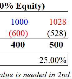
3. Leverage. Finally, leverage sits behind the other two drivers but can also operate on its own. Debt is a fixed contractual claim, meaning it does not rise with the company’s market value. Equity, however, captures all the upside once debt is repaid. The less equity the sponsor puts in upfront, the greater the share of eventual gains he can capture percentage-wise, assuming the company performs well.

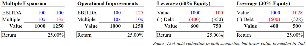
For instance, the table below shows how all three return drivers can, in theory, generate the same percentage return. The difference is that each one relies on a different lever, and the sponsor’s focus shifts accordingly. With multiple expansion, the emphasis is on making the company attractive enough for a buyer to pay a higher multiple. With operational improvements, the focus is on boosting profitability through better management and efficiency. And with leverage, the focus is on contributing as little equity as possible, so that even a modest increase in company value translates into a disproportionately higher gain for equity holders.

BEST CANDIDATES FOR LBOs

The best targets for an LBO usually share one or more of the following traits:

1. The company is undervalued (or can be purchased below its true intrinsic value).

2. Predictable and high free cash flow with a defensible competitive.

3. Strong management team.

4. Clear exit opportunity (e.g., a potential IPO).

5. A fragmented market, which allows for a roll-up strategy.

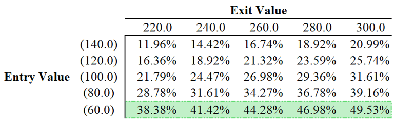
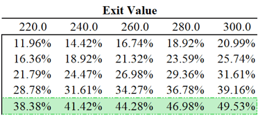
Still, if only one factor had to be picked above all others, it would be entering at the right price. Being undervalued at entry, and ideally bargaining down the acquisition price, is the single most powerful driver of returns. For instance, in the example below (shown in green), an entry at 60 produces a higher IRR than entering at 80, 100, 120, or 140—regardless of the eventual exit value. The only exception is the case of entering at 80 and exiting at 300, which yields slightly more than entering at 60 and exiting at 220. But such a $300 exit represents an extremely bullish upside scenario and should be treated with caution. This is why, in practice, price negotiations at entry are paramount.

As a side note, competitive position - often described as a “moat” (as coined by Warren Buffett) - gives sponsors confidence that cash flows will remain durable over time. This defensibility can take different forms: recurring revenue models, entrenched customer relationships, high switching costs, or strong brand recognition. Ideally, the industry backdrop also supports stability, with secular growth trends and limited exposure to disruptive technologies that might erode profitability.

HOW MUCH DEBT CAN A LEVERAGE BUYOUTS SUSTAIN?

Lastly but not least, many might ask themselves how much leverage a company can actually sustain. There is no single answer. Academia has long debated the “optimal capital structure” and the point at which lenders begin asking for more compensation as they move closer to equity risk. To keep things simple, I’ll break this into three parts: (1) cash flow capacity, (2) valuation buffers, and (3) how lenders price risk.

1) Cash Flow Capacity

The first lens is straightforward: can the company generate enough cash flow to service the debt? If not, it risks missed payments and will be forced to sit down with creditors for amendments. ake a simple example. Suppose a company has $200 of free cash flow available for debt service. At an 8% interest rate, that would support $2,500 of debt ($2,500 * 8% = $200). But in practice no lender will lend to the very limit, since cash flows fluctuate. They will leave a buffer. So instead of $2,500, maybe they cap the loan at $1,500. If the company has $400 EBITDA, this works out to 3.75x leverage ($1,500 / 400). This “buffer” is what allows the company to survive volatility without constant waivers or forbearance from creditors.

2) Valuation Buffer

The second lens is balance-sheet based: what is the value of the business? Lenders want to know that assets are worth more than liabilities, leaving equity as a cushion. If a company has $100 in assets and $80 in debt, creditors have a $20 cushion provided by equity. If assets fall to $70, creditors are impaired and would only recover 87.5% ($70 / $80). The thinner the equity cushion, the more exposed creditors are. This is why lenders rarely push leverage to the absolute limit. Different creditors also price this buffer differently. Senior lenders want a wide cushion and settle for lower returns. Subordinated or mezzanine lenders accept a thinner cushion but demand higher returns to compensate.

3) Pricing of Risk

The third lens is how lenders translate all of this into pricing. At the end of the day, debt is not just about capacity or value, it is also about risk and return. We will return to this idea in the following chapter on capital structure theory. For now, it is enough to note that the pricing of risk is fundamentally tied to the possibility of lenders losing money - that is, the risk of a default event.

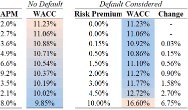
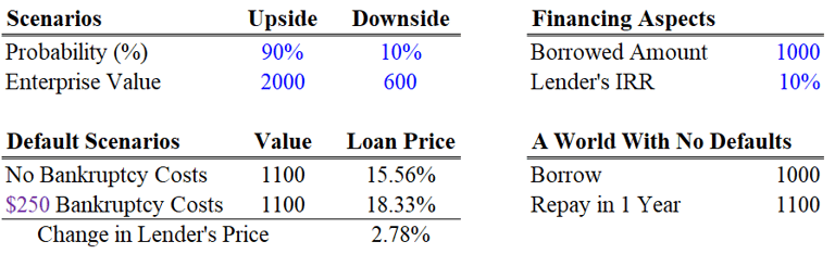
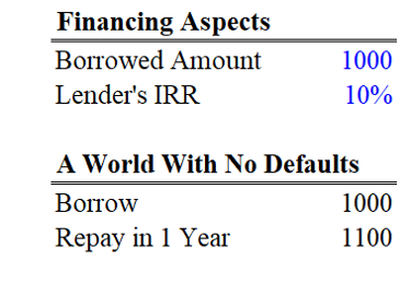
Let's see an example on this. Let’s assume the probability of an upside is 90% and the downside 10%. In the upside case, the firm is worth 2,000; in the downside, 600. The sponsor therefore sees an expected value of 1,860 (2,000 90% + 600 * 10%), which justifies pursuing the investment. For the bank, however, the calculation is different. Suppose it lends 1,100. The bank wants to earn an expected yield of 10%, meaning its expected payoff should be 1,210. To reach that, the loan must actually be priced at 15.5%. That extra 5.5% above the base yield is the credit risk premium. The higher the chance of default as leverage increases, the larger this premium becomes. This is shown below.

4) Capital Structure Trade-Off

This idea of the credit risk premium naturally extends into discussions about capital structure. The traditional theory goes something like this: the more debt you add, the cheaper the cost of capital becomes. Debt is cheaper than equity because (i) lenders usually require a lower return than equity holders, and (ii) in most tax codes, interest is tax-deductible, which effectively lowers its cost even further. This is why, in theory, firms should keep adding debt and drive down their overall cost of capital, a concept known as the Weighted Average Cost of Capital (WACC).

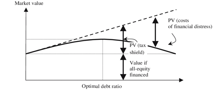
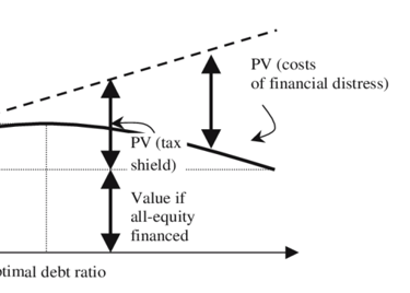
But this neat picture only works if we assume away the possibility of default. In the real world, once debt reaches a certain level, the risk of financial distress increases, and with it, the credit risk premium (which we showed above). Lenders begin demanding higher yields to compensate for the greater chance of loss. At the same time, the firm itself may face indirect bankruptcy costs i.e., legal fees, administrative burden, management distraction, even reputational damage, all which reduce the effective value of the business. So instead of the WACC curve endlessly falling as more debt is added, the line eventually bends back upward. Initially, leverage lowers the cost of capital because debt is cheaper than equity. But past a certain point, the rising cost of debt, driven by credit risk premia and the threat of distress, more than offsets the tax benefits. The result is a U-shaped curve, with a theoretical “optimal capital structure” somewhere in the middle. This is shown in almost all Corporate Finance literature, the so-called famous Modigliani Miller theory:

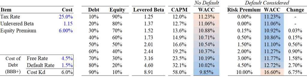
Now, an easier example can also be shown below where, for instance, the 'No Default' WACC shows this theory. However, when we we add the default risk (and hence the credit risk premium), the WACC becomes "richer" as our debt proportion in the capital structure raises past a certain level. As such, as more debt increases our WACC, we would settle that something around 40% debt would be our optimal capital structure as at that point our WACC is the lowest at 10.86%.

This concludes Part I. In Part II, we will turn from the broad theory to the instruments themselves, breaking down the different types of debt that make up the typical capital structure of an LBO.